Theory

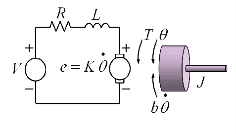
The DC motor dynamics:
The DC motor dynamics are represented by the following equations:
Mechanical equation:

$$ J\dot{\omega}(t)+K_f \ {\omega}(t) = K_m \ i(t) \tag{1}$$

where, J is the motor inertia, K_f is the damping coefficient, K_m is the motor constant, ω(t) is the angular speed of the motor, i(t) is the armature current, E _b (t) is the back electromotive force, given by E _b (t) = K _b ω(t), and K_b is the back EMF constant.

Electrical equation:

$$ L \dot{i}(t)+R {i}(t) + E_b (t)= V(t) \tag{2}$$

where, L is the inductance, R is the resistance, i(t) is the armature current, V(t) is the armature voltage (input).

Transfer Function:

$$ G(s) = \frac{\omega(s)}{V(s)} = \frac{K_m}{JL s^2 + (JR + LK_f) s + (RK_f + K_mK_b)} \tag{3}$$

Pulse Transfer Function:

The bilinear transform is used to transform continuous-time system representation to discrete-time.

$$ s = \frac{1}{T} ln(z) $$

$$ \approx \frac{2}{T} \frac{z -1}{z+1} $$

$$ \approx \frac{2}{T} \frac{1- z^{-1}}{1+z^{-1}}\tag{4} $$

where T_s is the sampling period.

$$ G(z) = \frac{\omega(z)}{V(z)} = \frac{(z^2+2z+1)K_m}{z^2[\frac{4JL}{{T_{s}}^2}+\frac{2(LK_f+RJ)}{T_{s}}+(RK_f+K_mK_b)]+z[2(RK_f+K_mK_b)-\frac{8JL}{{T_{s}}^2}]+[\frac{4JL}{{T_{s}}^2}-\frac{2(LK_f+RJ)}{T_{s}}+(RK_f+K_mK_b)]} \tag{5}$$

$$ G(z) = \frac{\omega(z)}{V(z)} = \frac{(K_m+2K_mz^{-1}+K_m z^{-2})}{[\frac{4JL}{{T_{s}}^2}+\frac{2(LK_f+RJ)}{T_{s}}+(RK_f+K_mK_b)]+z^{-1}[2(RK_f+K_mK_b)-\frac{8JL}{{T_{s}}^2}]+z^{-2}[\frac{4JL}{{T_{s}}^2}-\frac{2(LK_f+RJ)}{T_{s}}+(RK_f+K_mK_b)]} \tag{6}$$

State Space Model of the DC motor:

Continuous State Space form:

$$ \begin{bmatrix} \dot{\omega}(t) \newline \dot{i_a}(t) \end{bmatrix} = \begin{bmatrix} -\frac{K_f}{J} & \frac{K_m}{J} \newline -\frac{K_b}{L} & -\frac{R}{L} \end{bmatrix} \begin{bmatrix} \omega(t) \newline i_a(t) \end{bmatrix} + \begin{bmatrix} 0 & \frac{1}{J} \newline \frac{1}{L} & 0\end{bmatrix} \begin{bmatrix} V_a(t) \newline T_d (t) \end{bmatrix} \quad $$

$$ y(t) = \begin{bmatrix} 1 & 0 \end{bmatrix} \begin{bmatrix} \omega(t) \newline i_a(t) \end{bmatrix} \quad $$ $$ \tag{7} $$

where, T_d is the load disturbance.

Discrete state space form represented by the following equations:
State equation:

$$ {x}[k+1]=F x[k]+g u[k] \tag{8a} $$

Output equation:

$$ y[k] = C x[k] \tag{8b} $$

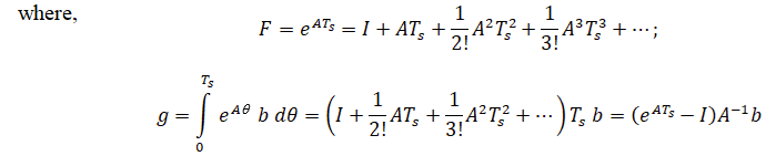
Discrete State Space form:

$$ \begin{bmatrix} \omega [k+1] \newline i_a [k+1] \end{bmatrix} = \begin{bmatrix} 1-\frac{K_f T_s}{J} & \frac{K_m T_s}{J} \newline -\frac{K_b T_s}{L} & 1-\frac{R T_s}{L} \end{bmatrix} \begin{bmatrix} \omega [k] \newline i_a [k] \end{bmatrix} + \begin{bmatrix} \frac{K_m {T_s}^2}{2JL} & (\frac{T_s}{J}-\frac{K_f{T_s}^2}{2J^2}) \newline (\frac{T_s}{L}-\frac{R{T_s}^2}{2L^2}) & -\frac{K_b {T_s}^2}{2JL} \end{bmatrix} \begin{bmatrix} V_a(k) \newline T_d (k) \end{bmatrix} \quad $$

$$ y[k] = \begin{bmatrix} 1 & 0 \end{bmatrix} \begin{bmatrix} \omega[k] \newline i_a[k] \end{bmatrix} \quad $$ $$ \tag{9} $$